Project: the Automatic #plotloop Machine

What’s this?

I recently built an “Automatic #plotloop Machine”, named after the common social media hashtag for these animations made of individually plotted frames. This article is a thorough description of the project, covering both hardware and software aspects.

First, here is a video:

So, this is all very nice, but why does this article need to be more than six thousand five hundred word long?! Sure, the machine’s neat, but it’s not like everyone wants to make one, right?

Well, in the making of this project, I found myself using a number of tools and techniques which, I think, might be of more general interest—that is, also for someone without aspirations for maximally complex animation production methods.

Rather than the seasoned maker, who might more efficiently fill knowledge gaps with a few targeted Google queries, I wrote this article for the many people in the plotter space with an artistic rather than technical background. I’m hoping this article might provide some technical baggage to fuel their tinkering urge, which, being involved with plotters, they obviously have.

So, if any or all of the following topics sound like they might be useful, have a read!

• How to use a Raspberry Pi to automate things like taking pictures or controlling stepper motors?
• How to mate a stepper motor with LEGO Technic contraptions?
• How to efficiently control a RPi via ssh?
• How to efficiently control a RPi using a web framework?
• How to use vsketch to produce plot loops (automated or otherwise)?
• How to use doit to automate complex workflows?
• Etc.

This article is not a beginner tutorial either. A number of the topics covered here would, in tutorial form, warrant an even longer treatment by themselves. There should be enough information to understand how things work and understand the relevance of the tools I’ve used. Actually applying them in a project may, however, require some more focused reading. Likewise, the code is what I’d call “project quality”—it does the job, I’m not too ashamed of it (mostly), but shouldn’t be construed as top-notch, state-of-the-art, production-ready copy-paste material.

Overview

Here is how the setup looks like in on my mobile plotting station:

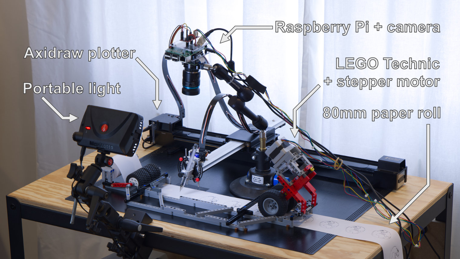
Here are the main components involved:

1. An AxiDraw SE/A3 from Evil Mad Scientist Laboratories, driven by a Raspberry Pi 4 not visible in the picture (it’s neatly installed in the lower section of the plotting station).
2. A Raspberry Pi 3 hooked to the High Quality Camera module and a EasyDriver stepper motor driver, held by a Manfrotto 241s Pump Cup and 244 Mini Friction Arm.
3. An 80-mm paper feeder contraption made of LEGO Technic and a stepper motor.
4. A Manfrotto ML840H On-Camera LED light, held by a couple of umbrella swivel adapters and a Phottix Multi Clamp.

Clearly, having a bunch of photography-related gear around is convenient for this kind of project! 😄

Here is a schematics view of the same setup:

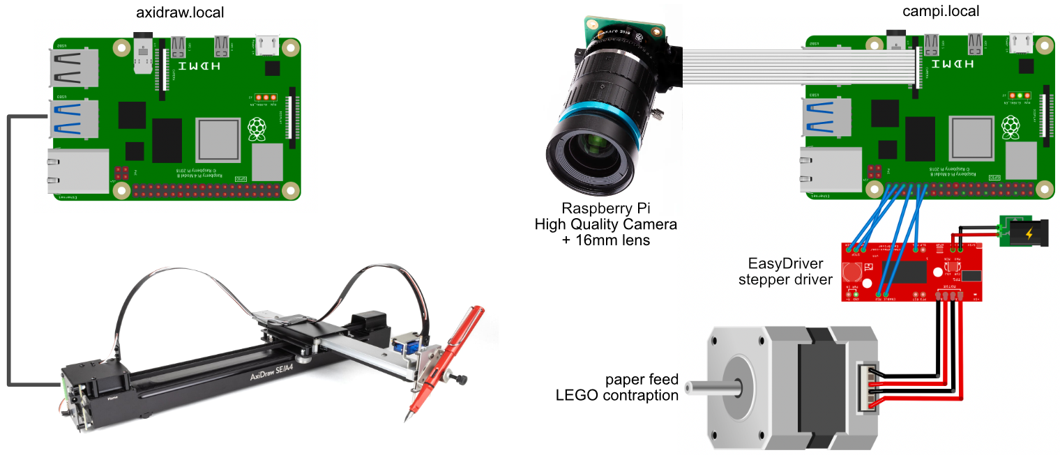
The most salient aspect is the use of two Raspberry Pis. This is entirely unnecessary—a single RPi would be entirely sufficient. This arrangement happened to be more convenient for me because my plotting station already includes a RPi (with hostname axidraw.local) for my day-to-day use of the AxiDraw.

Missing from both pictures is my computer, which I use to generate the frames and controls the plotting process by sending orders to both RPis via Wi-Fi.

In the next sections, I will dig into the details of many hardware and software aspects of this setup, culminating with the doit script which orchestrates everything ranging from generating the frame data, creating a simulated animation, controlling both RPis for plotting and picture acquisition, and assembling the final GIF:

Hardware

Camera

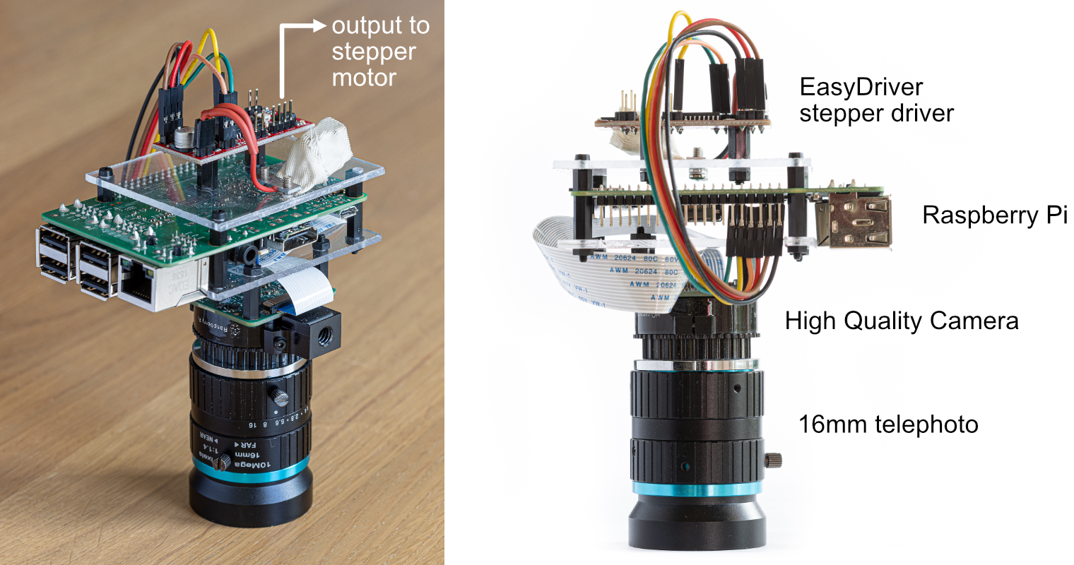
The camera assembly includes a Raspberry Pi (with hostname campi.local), the camera module and its optics, as well as the stepper motor driver. The three boards are assembled together using custom-cut plexiglass plates and nylon spacers. The camera module is connected to the RPi’s camera interface using the provided 200mm ribbon cable.

I chose the High Quality Camera for the following reasons:

• It is made by the Raspberry Pi Foundation itself, so it has best-in-class software support out-of-the-box.
• With 12 megapixels and a large pixel size, it is one of the highest quality camera available for the Raspberry Pi.
• It uses interchangeable, C-mount lenses, which means that I can use a lens that’s best suited for this setup.

For the lens, I selected the 16mm telephoto. With its relatively narrow field of view, it minimises the distortions and can be placed high enough to leave space for the plotter to operate. With this lens, the positioning is mainly driven by the minimum focus distance, which is approximately 24cm, measured from the front-most part of the lens.

Here is a sample frame and the corresponding raw image as taken by the camera (high-res version):

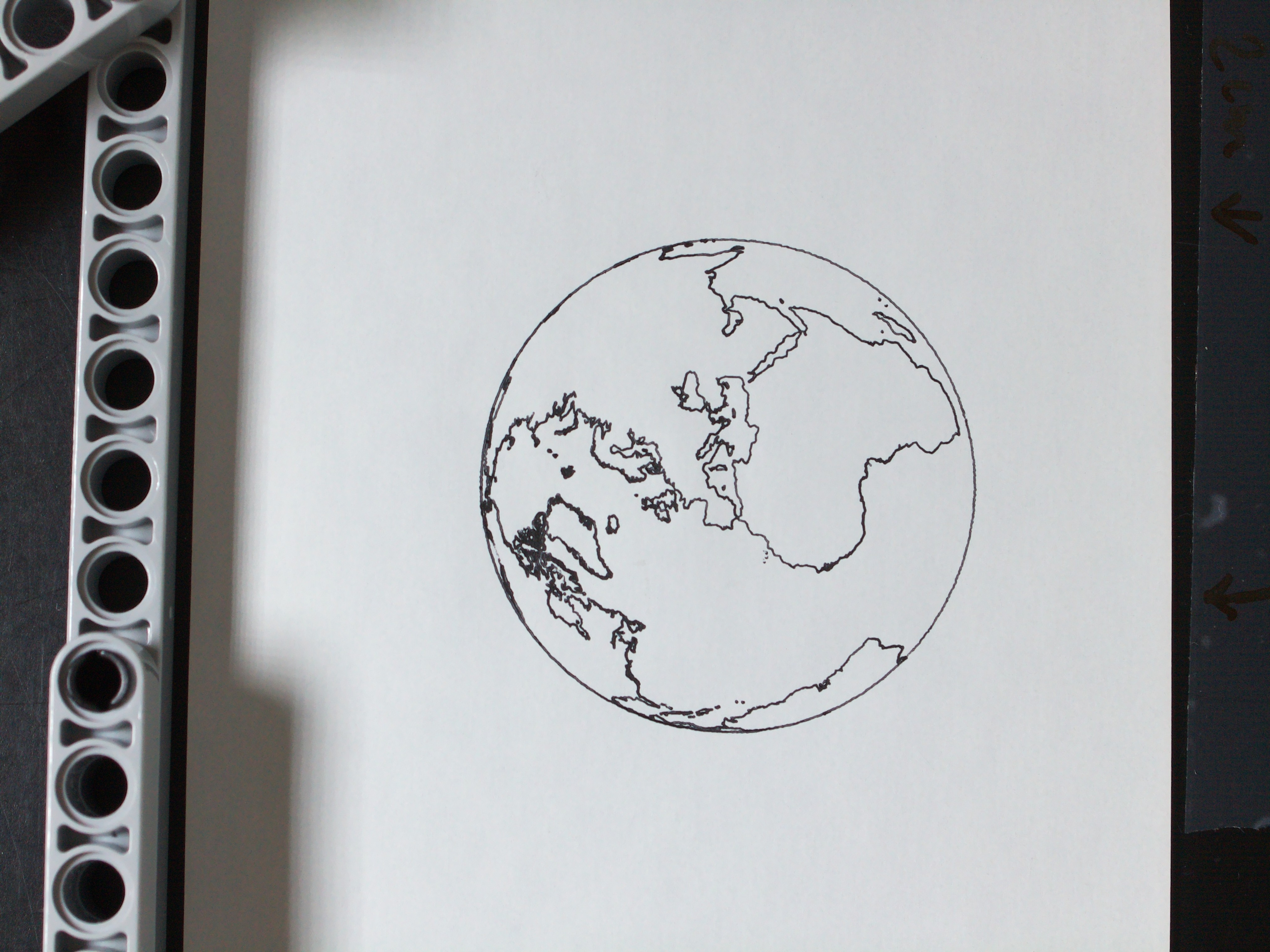
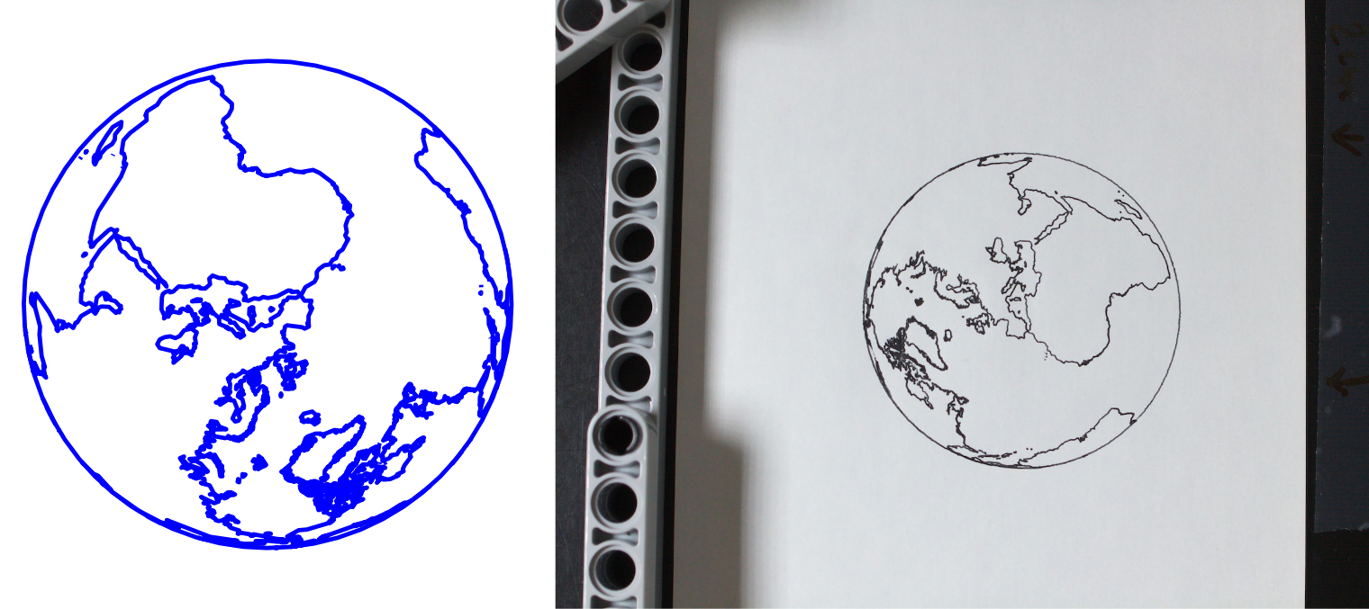
Note that the image is rotated by 90° compared to the actual frame. It just happened to be easier to set up the camera this way. It will be automatically corrected before the final animation is assembled.

Stepper motor driver

The campi.local RPi is also in charge of driving the paper feeder’s stepper motor via an EasyDriver board. As their name imply, stepper motors divide their full rotation into a number of discreet, equal steps. This makes them very convenient for use cases where accuracy and reproducibility is important, like 3D printers, plotters, and… makeshift paper feeders. Stepper drivers generate the high power electrical signals needed to run the motor based on a simple GPIO inputs.

Here is a close-up of the wiring schematic:

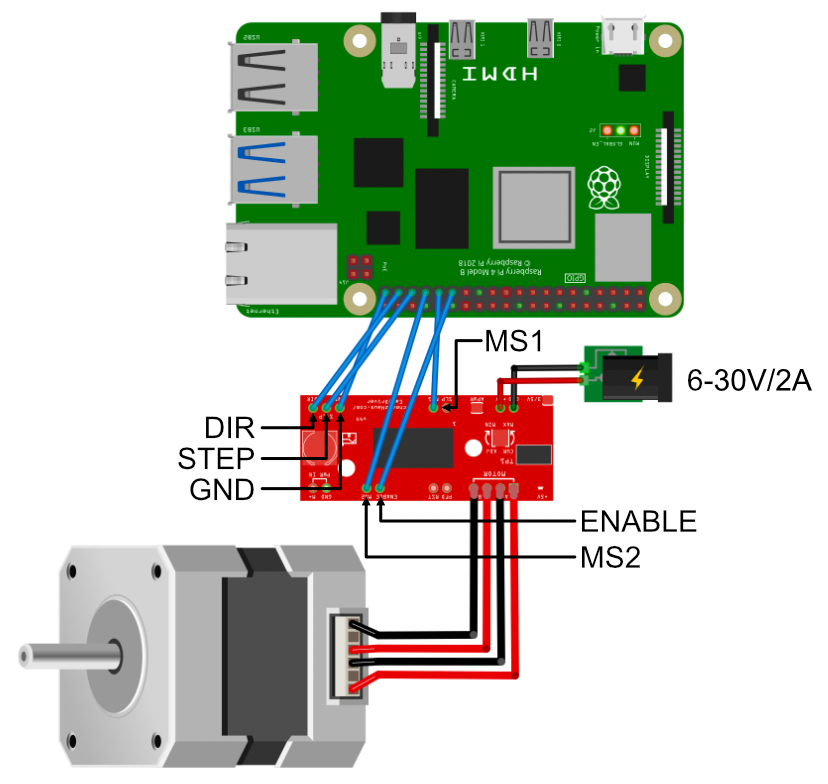
The main inputs are STEP and DIR. The motor turns by one step for each STEP pulse (transition from 0 to 1), while the rotation direction is controlled by DIR.

The ENABLE input controls whether the motor outputs are powered or not. When they are, the driver actively keeps the motor in its position, which tends to heat both the driver and motor itself. As the feeder spends most its time waiting for the plotter to draw the frame, it is good idea to drive ENABLE only when actually running the feeder.

The MS1 and MS2 inputs control the so-called “micro-stepping” capability of the driver. This feature increases the accuracy of the motor by further dividing the motor’s physical steps into up to 16 micro-steps. For a low-precision paper feeder like mine, this is not useful and the wiring can be skipped¹.

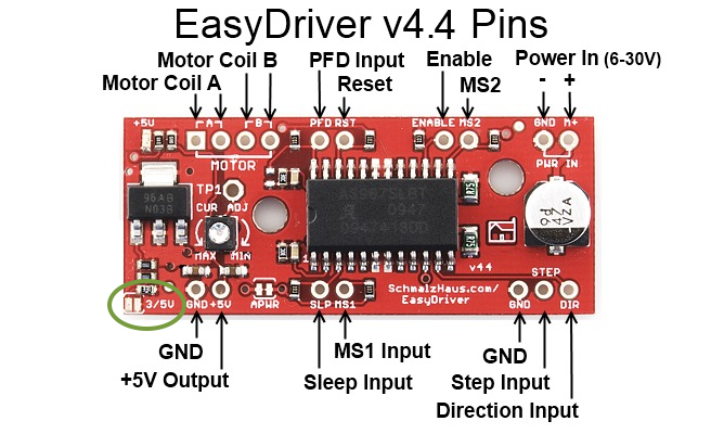
One nice feature of the EasyDriver board is the ability to choose either 3.3V or 5V GPIO voltage. The default is 5V, but since the RPi uses 3.3V, I set the board to this voltage using a small solder bridge over the pads at the very bottom left of the board:

LEGO structure

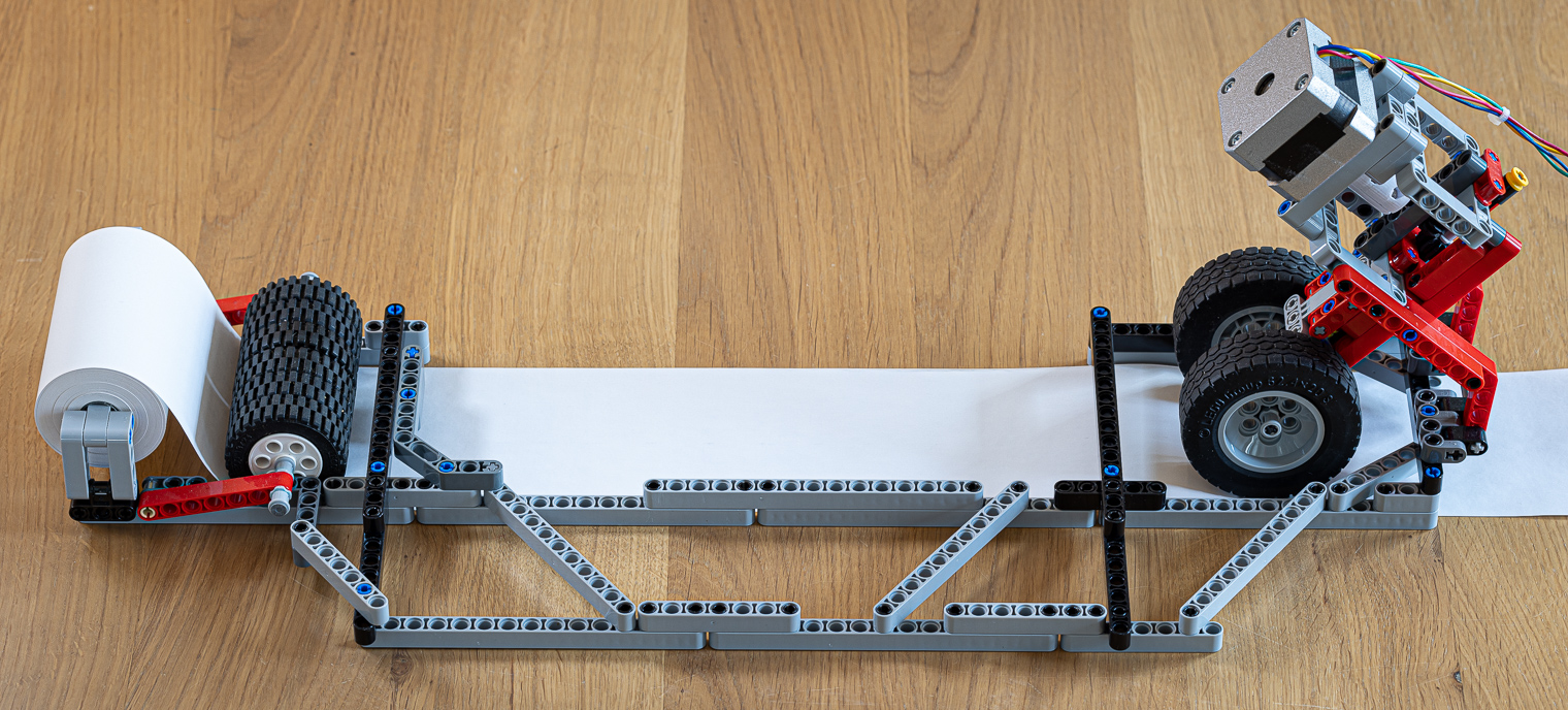
My LEGO building skills aren’t anything to boast about—a skilled builder would likely do a much better job. Yet, my contraption turned out to work rather reliably thanks to a few key design decisions.

Most importantly, I wanted to leave the feeder “open” on the “top” side to minimise the chance of collision with the plotter or the pen during operations. The lower parallel structure is thus designed to maintain some rigidity between the paper roll part and the feed part. This actually worked much better that I anticipated!

These structures are really easy to build once your remember that 3² + 4² = 5²:

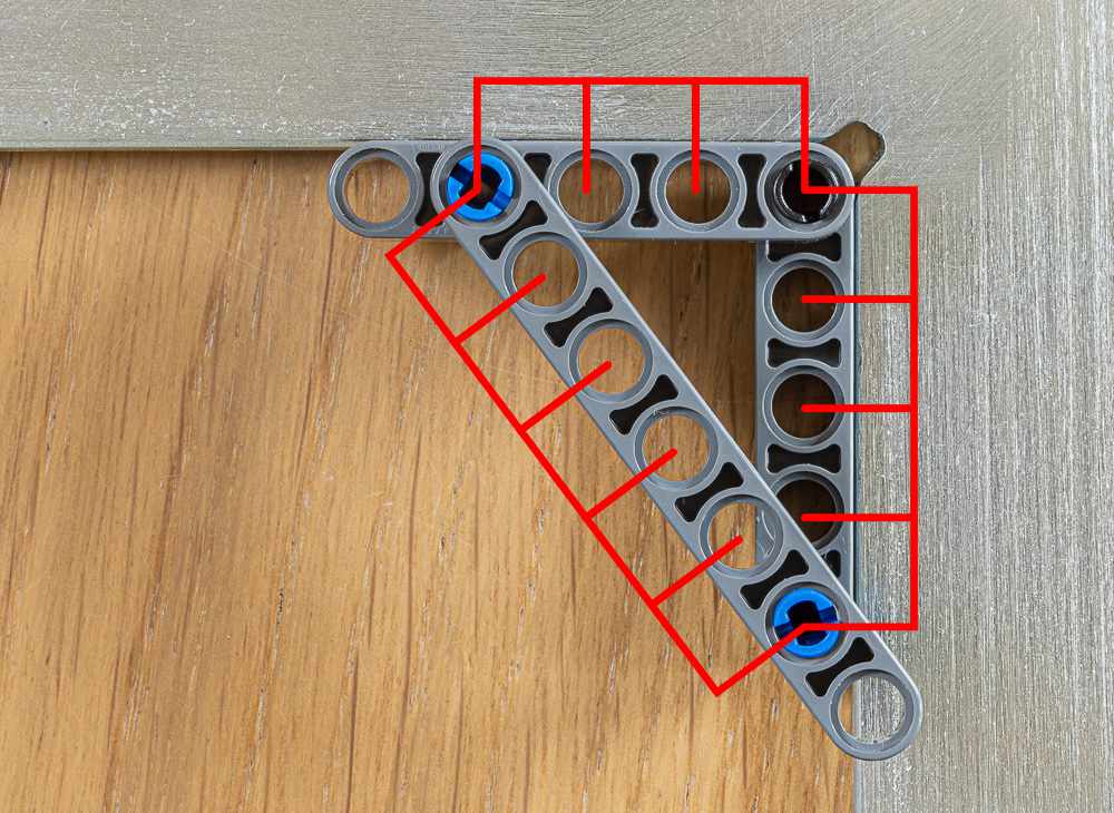
All my diagonals use this arrangement and provide rigidity to the structure (purely rectangular structures are prone to parallelogram deformation).

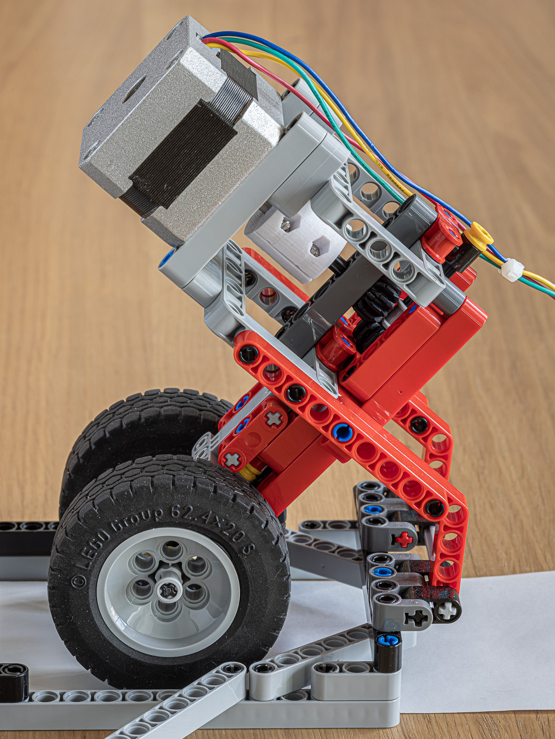
Using the stepper motor weight to put pressure on the feeding wheel was another successful design. This ensured practically no paper slippage.

Finally, remembering that the LEGO stud pitch is 8mm, a 10-stud distance is a good fit for 80mm paper rolls. These are easy to source in office supply shops.

Stepper-LEGO integration

One might wonder why I used a custom stepper motor instead of native LEGO motors to drive the feeder. The decision boils down to two issues with LEGO motors:

1. There are no stepper-type LEGO motors, so their accuracy is not great, nor is their power.
2. Interfacing LEGO motors to a RPi is more complicated than using a stepper motor (especially if you already have stepper drivers lying around).

I actually tried to use a LEGO Mindstorm motor initially. I used a BrickPi board to interface the motor to the RPi. It worked, but as noted above these motors are not ideal for the task and ended up not being precise and reliable enough.

An alternative to the BrickPi board would be to use the actual Mindstorm controller. This is not ideal though, as the controller is battery powered and must be tinkered with to accept external power. Also, the RPi must connect to it via Bluetooth, and a specific Python package must be used.

All in all, in my experience, using a stepper motor is just easier.

This begs the question of how to physically interface the stepper motor with LEGO Technic parts.

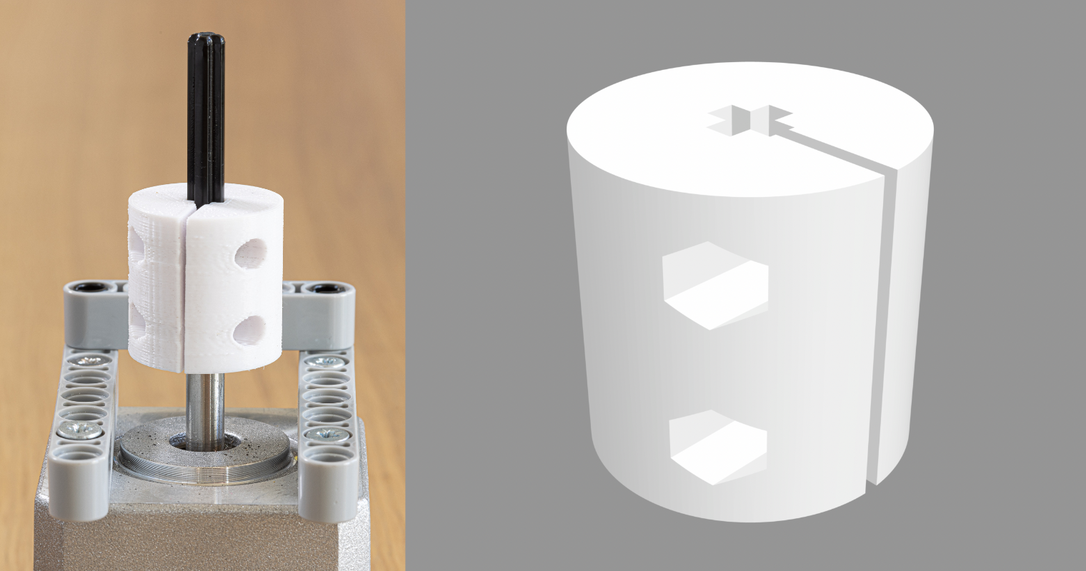
I used a 3D-printed adapter of my own design to interface the 5mm axle of my motor to Technic axles. There are many such designs available online for various shapes and sizes of motor axles.

It turns out that physically assembling the motor with LEGO Technic is easy enough when using the NEMA 17 form factor (one of the most commonly used by makers). The offset between their M3 attachments is 31mm. This is close enough to the 32mm offset between two 3-stud-apart Technic holes. Using conic screws easily takes up the remaining 1mm difference:

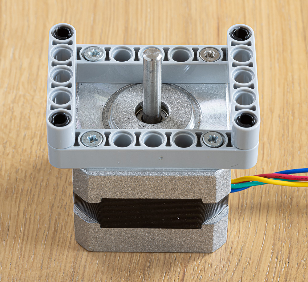
Crucially, this method keeps the motor axle properly aligned with the Technic grid.

Software

Setting up the Raspberry Pi for friction-less SSH

There is ample documentation available online on how to setup Raspberry Pis, which I won’t reproduce here. I’d like to focus instead on how to configure the RPi such as to minimise any friction when interacting with your RPi via SSH—either manually or automatically.

Here is what’s needed to achieve this:

1. Unless you are using wired Ethernet, your home Wi-Fi must be configured on the RPi (of course, duh).
2. SSH must be configured for key-based authentication. This removes the need to input a password when SSHing into your RPi, which is annoying with manual operations and precludes automation.
3. ZeroConf/Bonjour/Avahi is installed and active. This means that you can connect to the RPi using a URL in the form of hostname.local instead of using an explicit IP address, which is hard to remember and subject to change.
4. You computer must “know” which username to use when connecting to a given RPi.

For key-based authentication, you must first generate a public/private key pair on your computer (if you haven’t done so already). This is done using the following command:

ssh-keygen

You’ll need to answer a few questions, which can all be left as default. This will create two files in your home directory:

• The private key: ~/.ssh/id_rsa
• The public key: ~/.ssh/id_rsa.pub

(Actual naming may differ depending on the type of key generated.)

The idea is to provide your public key (this is important—not the private key!) to the RPi so that it can accept connections without requesting a password when the originator possesses the corresponding private key.

Most of the configuration, fortunately, is addressed by the official Raspberry Pi Imager, which I strongly suggest using. Everything can be set in the “Advanced Options” dialog, including the hostname, the SSH public key, and the Wi-Fi credentials:

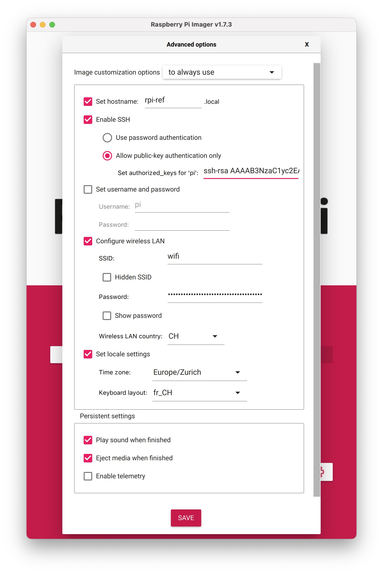
Again, note that the content of your public key (~/.ssh/id_rsa.pub) should be pasted in the relevant field.

Finally, you need to tell your computer’s SSH that user pi (or whichever you chose) should be used by default when connecting to the given RPi. Create the ~/.ssh/config file if needed, and add the following content:

Host axidraw.local
    User pi

This tells your computer’s SSH to default to the username pi whenever it connects to axidraw.local.

If you already have a working RPi image, and you don’t want to recreate one from scratch, you can do the same configurations manually as follows:

• Check this article for Wi-Fi configuration.
• For key-based SSH authentication, create or edit the ~/.ssh/authorized_keys2 file on the RPi and add the content of your public key on a new line.
• Install ZeroConf/Bonjour/Avahi support with sudo apt-get install avahi-daemon.
• Change the hostname by running sudo raspi-config. The configuration is in the Network Options menu.

Here are the cool things that you can now do remotely without entering a password:

scp file.svg axidraw.local:          # copy a local file to your remote user directory
scp file.svg axidraw.local:files/    # copy a local file the remote ~/files/ directory
scp axidraw.local:files/file.svg ./  # copy a remote file locally

ssh axidraw.local     # log to your remote RPi
ssh axidraw.local ls  # list the files in your home directory

cat my_file.svg | ssh axidraw.local axicli -L 2 -d 37 -u 60 -N -m plot   # plot a file!

This last one is particularly nice. SSH allows you to pipe the output of a local command (here cat just outputs the contents of my_file.svg) into a remote command’s input. This is a very powerful combination that I use for this project.

Controlling the camera and the feeder

The campi.local Raspberry Pi has two missions: taking a picture of the frame after it is drawn, and run the motor to feed blank paper for the next frame. One of the easiest ways to make these functionalities remote controllable is to run a small HTTP server with two end-points, one for each task.

This is really easy to do with FastAPI (Flask would also work just as well). The corresponding code is available here, along with a requirements.txt file listing the required packages.

Taking pictures

For illustration, here is a shortened version with only the image acquisition part:

from fastapi import FastAPI
from fastapi.responses import FileResponse
from picamera2 import Picamera2

# create a FastAPI server
app = FastAPI()

# setup and start the Pi camera for still frame acquisition
picam2 = Picamera2()
still_config = picam2.create_still_configuration(controls={"ExposureValue": 0})
picam2.configure(still_config)
picam2.start()

# create a GET endpoint accepting a "ev" parameter and returning a JPG file
@app.get("/img/")
def get_picture(ev: int = 0):
    picam2.set_controls({"ExposureValue": ev})
    array = picam2.capture_file("/tmp/temp.jpg")
    return FileResponse("/tmp/temp.jpg", media_type="image/jpeg")

All it takes to run the server is to the following command:

uvicorn campi:app --host campi.local --port 8000

Uvicorn is a web server implementation fo Python uses FastAPI (in our case) to handle web requests. Here, campi:app tells Uvicorn to use the app object in the campi module (assuming our file is named campi.py).

Note in passing how having ZeroConf setup with the RPi means that, once again, we don’t need to mess with explicit IP addresses. (Here, specifying a --host other than the default localhost is required to allow another computer to access the server.)

With the server running, any other computer on the local network can acquire a photo using the following command:

curl -s -o /tmp/test.png campi.local:8000/img/?ev=1

A couple of learnings from the field:

• Like in the example above, I’m using an exposure value of +1 with the #plotloop machine. This is because the white paper tend to lead to underexposure. With the code above, this parameter doesn’t seem to have effect until after the second picture is taken. So, after starting the server, I always use the command above to have one picture taken with ev=1 so the camera is primed when the machine actually uses it.
• The server can run for a long time, taking multiple hundreds of pictures (the rotating earth loop is 280-frame long). So it’s pretty important that the /img/ end-point doesn’t leak any memory. Especially uncompressed-frame-sized buffers. I actually ran into this issue with the first implementation, which used a memory buffer instead of a temporary file. After messing with tracemalloc for a while to figure this out, it ended up being just easier to switch implementation. For my first loop with the machine, the leak would fill my RPi’s memory and crash every 20 images or so—it was painful process to go through the whole loop!

Moving the motor

I use another end-point to control the feeder motor. This time, it includes a mandatory parameter in the URL: the approximate number of centimetre of paper to feed. Here is how it looks in the code:

@app.get("/motor/{cm}")
def run_motor(cm: int):
	...

Using this end-point is as easy as:

curl -s campi.local:8000/motor/5

The implementation is really boring. The gist of controlling a stepper motor is to toggle a GPIO up and down as many times as needed—one per step. This could easily be done manually, but I’m using RpiMotorLib to reduce the code to a single line. The conversion from centimetre to step count depends on your motor (mine has 400 steps per full rotation, which is fairly standard) and the feeder wheel size. I have a magic number in the code that I tuned by trial-and-error.

It’s worth noting that the accuracy of the feeder mechanisms is not critical for this machine because the paper isn’t moved at all between the frame being drawn and the picture taken. The feeder has thus no impact on frame-to-frame alignment—only the plotter’s repeatability matters here (which is a non-issue with the AxiDraw ❤️).

Another couple of things I learned on the way:

• As mentioned earlier, the motor and the driver can generate quite a bit of heat and power consumption when active, even when not moving. That’s why I manually toggle the ENABLE pin in the motor end-point. That way the motor is kept unpowered most of the time, and only activated when it must be moved.
• With the Raspberry Pi, it’s important to properly shut down the GPIO sub-system when exiting your program. It avoids some errors and minimise the risk for the hardware². The proper way to do this with FastAPI is to implement a shutdown event handler:

  @app.on_event("shutdown")
  def shutdown_event():
      GPIO.cleanup()
  

Using vsketch for plot loops

Unsurprisingly, I’ve used vsketch to generate the animation frames. Before diving into the actual sketch I made for this article, I want to shortly digress on how to structure a sketch to produce SVGs suitable for plot loops.

Here is a simple example of a plot loop sketch:

import math
import vsketch

class PlotloopSketch(vsketch.SketchClass):
    frame_count = vsketch.Param(50)
    frame = vsketch.Param(0)

    def draw(self, vsk: vsketch.Vsketch) -> None:
        vsk.size("5x5cm", center=False)
        vsk.scale("cm")

        radius = 2
        vsk.circle(2.5, 2.5, radius=radius)
        angle = 360 / self.frame_count * self.frame
        vsk.circle(
            2.5 + radius * math.cos(math.radians(angle)),
            2.5 + radius * math.sin(math.radians(angle)),
            radius=0.1,
        )

    def finalize(self, vsk: vsketch.Vsketch) -> None:
        vsk.vpype("linemerge linesimplify reloop linesort")

This sketch (available in the vsketch repository) animates a small circle rotating around a larger circle³:

The first noteworthy aspect is its use of the two parameters: frame_count and frame. This makes it super easy to control the animation length and generate all the frames. For example, the frames for this GIF were generated with the following command:

vsk save plotloop -m -p frame_count 13 -p frame 0..12

(Note the use of -m to use all available CPU cores.)

Another key element is to use center=False in the initial vsk.size() call. Without this, vsketch would auto-centre every frame based on the geometry and this would result in the animation wobbling around. I actually made a similar mistake with one of my first plot loop⁴:

Last but not least, notice how the algorithm generates the exact same frame for frame = 0 and frame = frame_count⁵. This is obviously necessary to obtain a properly looping behaviour—but is easier said than done for all but trivial examples.

One way is to use periodic trigonometric functions such as sine and cosine like I did in the example above. This is also the approach I used for the rotating Earth loop.

Many generative artwork rely on Perlin noise. Some implementations may offer some kind of periodicity that could be used to generate a looping set of frames. Alternatively, periodicity can be achieved by sampling the noise field along cylindrical coordinates instead of on a cartesian grid.

An entire article could be written on this topic, and this one is long enough. Instead, I’ve added another example to the vsketch repository to illustrate this principle:

The rotating Earth sketch

The full sketch code is too long to be reproduced in this article—it’s available here in my sketches repository on GitHub. Instead, I will provide here an overview of how it’s implemented. You might want to open the code in another window to follow along.

Data preprocessing

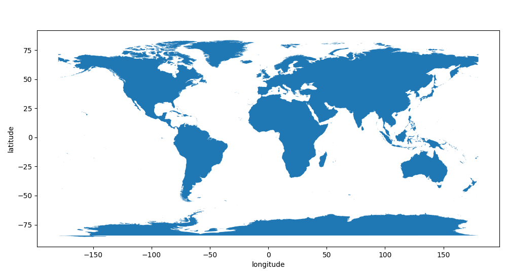
First, the data. I used the World Country boundaries from ESRI. It contains polygons for all countries in the world. By merging them with Shapely’s unary_union(), one can obtain the land/water boundaries. This happens in the build_world() function.

Here is how the merged countries look after the union step:

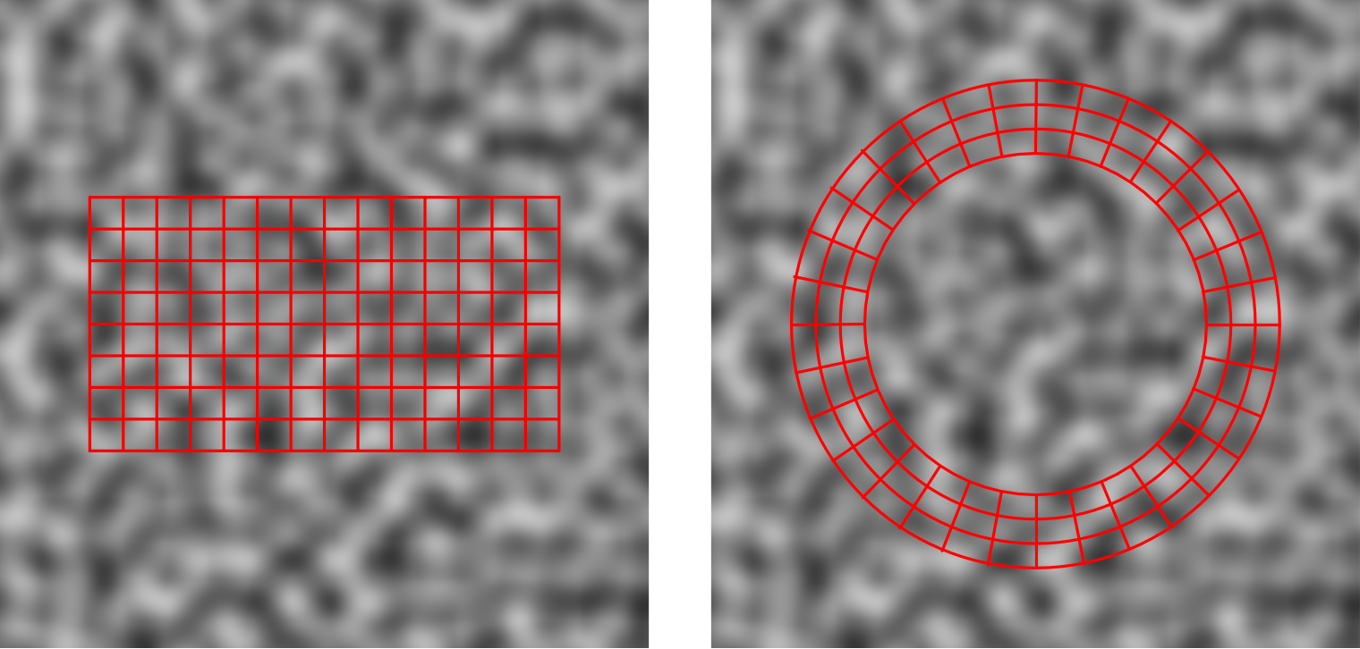
There is one oddity I had to deal with, which explains the magic numbers and other ugliness in that function: Antarctica. This is the only body of land sitting over one of the poles, which are singularities in the latitude/longitude coordinate system.

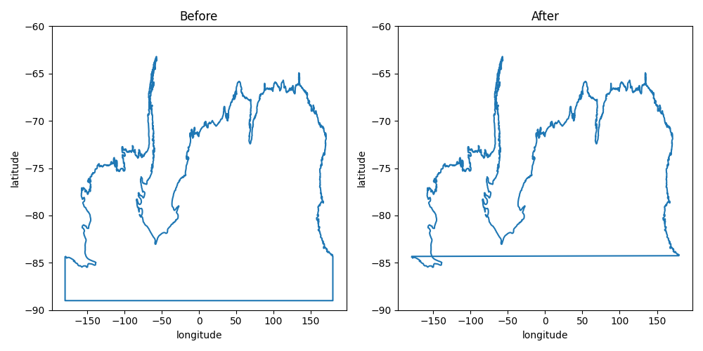
The left is how the data looked like originally. On the right is the boundary once the artificial limit at ~80°S is removed. In lat/long coordinates, it becomes a self-intersecting polygon. This can be dealt with a simple Shapely trick: create a LinearRing with the (self-intersecting) boundary and apply unary_union() on it. This creates a MultiLineString containing a corresponding list of non-intersecting linear rings.

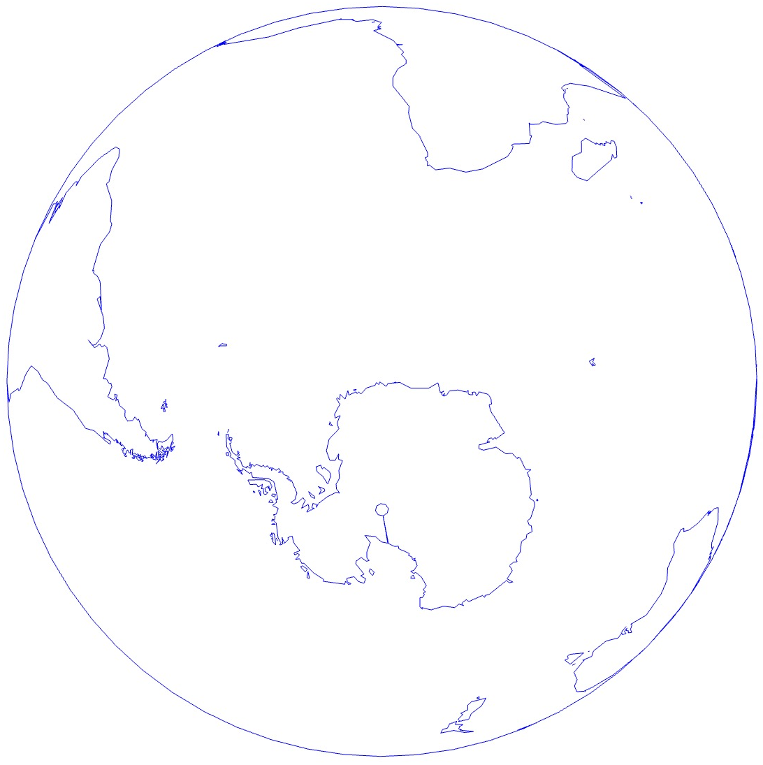
This is the glitch that this procedure solved:

Another important step is to filter land masses by area, to avoid the myriads of tiny isles that would clutter the result and massively increase plotting time. You can’t just use the .area attribute from Shapely with lat/lon coordinates as this isn’t an equal-area projection, so I shamelessly copy/pasted polygon_area() from StackOverflow.

The final preprocessing step consist of converting the lat/lon land boundaries (stored in a Shapely Polygon instance) into 3D points on the unit sphere (stored as a Nx3 NumPy array). This is done by the project_polygon() function. The projected boundaries are stored in the LINES global variable.

Rendering the Earth

The Earth rendering can be broken into the following steps:

1. Rotate the Earth data as needed.
2. Crop away the “far side” part of the data.
3. Project orthogonally the rest of the data, a.k.a. drop the coordinate along which the backside was cropped and use the other two for drawing.
4. Draw a circle :)

For rotation, I first compute 3 angles around the X, Y, and Z axes. These angles can be manually set for testing, or generated by trigonometric functions with different frequencies. Naturally, I make sure that these function are periodic with the frame count for a properly looping behaviour.

I then generate 3 rotation matrices:

rot_x = np.array(
    [
        (1, 0, 0),
        (0, math.cos(math.radians(rot_x_angle)), -math.sin(math.radians(rot_x_angle))),
        (0, math.sin(math.radians(rot_x_angle)), math.cos(math.radians(rot_x_angle))),
    ]
)
rot_y = np.array(
    [
        (math.cos(math.radians(rot_y_angle)), 0, math.sin(math.radians(rot_y_angle))),
        (0, 1, 0),
        (-math.sin(math.radians(rot_y_angle)), 0, math.cos(math.radians(rot_y_angle))),
    ]
)
rot_z = np.array(
    [
        (math.cos(math.radians(rot_z_angle)), -math.sin(math.radians(rot_z_angle)), 0),
        (math.sin(math.radians(rot_z_angle)), math.cos(math.radians(rot_z_angle)), 0),
        (0, 0, 1),
    ]
)

Finally, I combine them a single transformation matrix (did I mention I love NumPy?):

rot = rot_x @ rot_y @ rot_z

With that, rotating every single points of one of the land boundary line is just a matter of:

rotated_line = (rot @ line.T).T

Here, .T is used for transpose, and is needed for NumPy broadcasting rules to work. Remember that the actual calculation (3x3 matrix multiplication on every single points in line) happens in highly optimised C code, so this operation is fast.

Cropping is actually a bit trickier because you have to account for lines that may go from the front side to the far side and back, possibly multiple times. The cropping operation on a single line may thus result in multiple “sub-lines”.

Luckily, I had already sorted out most this for vpype’s crop command. vpype’s API includes the crop_half_plane() function, which crops a line at a give location along one of the X or Y axis⁶. Adapting it to the 3rd dimension was trivial. While copy/pasting the function, I took along _interpolate_crop(), which deals specifically with computing the intersection of a line segment with the cropping plane.

Once the land boundary lines are cropped along one dimension, it’s a matter of drawing them using the other two dimensions using vsk.polygons. Which dimension is used for what is not very important since we’re dealing with a sphere. I made it so that when rotation angles are set to 0, the (0°, 0°) lat/lon point (somewhere in the Atlantic ocean, off Ghana) is dead in the center of the rendered Earth.

In the sketch code, you’ll also find controls to enable pixelation using vpype-pixelart. I ran some trials with it but decided against it—to messy for this kind of line work.

Putting it all together with doit

At this point, all the #plotloop machine’s body parts are in place and just need a beating heart to set them in motion. doit is the perfect tool for this.

Although doit is rather easy to use, it still has a tiny bit of a learning curve. If this is your first ever encounter with it, you might want to check the introductory article I recently wrote. This project takes this to a whole new level.

Instead of looking at the dodo.py file line by line, I’ll first provide an overview of the workflows it implements (again, you might want to open the file in another window to follow along). Then, I’ll go deeper into a few, hand-picked topics to highlight interesting techniques.

The workflows

The bulk of the dodo.py file implements two workflows using a bunch of tasks: one is to create a simulated animation based on the frames' SVG, and another to plot, photograph, post-process, and assemble the frames into the final animation.

Here is a schematic of the workflows.

Let’s review the tasks involved in creating the simulated animation:

• The generate task generates all the frame SVGs with a single call to vsketch. It is basically running some version of this command:

  vsk save . -m -p frame_count 280 -p frame 1..280
  

  The outcome of this task is one SVG file per frame, numbered from 1 to 280.
• Each of the simframe:XXXX sub-task takes one frame SVG and convert it to a JPG with a _simulated prefix using librsvg’s rsvg-convert⁷. The sub-tasks are named after their corresponding frame number, e.g. simframe:0010 correspond to the frame number 10.
• Finally, the simulate task combines all the simulated frames into a single animated GIF, using ImageMagick’s convert command.

I’m calling this a workflow because each of these tasks have their file_dep and targets carefully defined. As a result, doit understands the dependency relationship between them. From a clean slate, calling doit simulate will first execute generate, then each of the simframe:XXXX sub-tasks, before finally running simulate to produce the animation.

The workflow for the actually plotted animation is similarly structured, but includes an additional post-processing step:

• The workflow starts with the same generate task as before.

• Each of the frame is then plotted and photographed by the corresponding plot:XXXX sub-task, which performs the following steps:

  • Plot the frame by sending the SVG via SSH to axicli running on the axidraw.local RPi (as described earlier).
  • Move the pen away by 3 inches to get it out of camera view (again, using SSH and axicli).
  • Take a picture of the frame and download the corresponding image using curl (as described earlier).
  • Move the pen back to its original position.
  • Feed fresh paper using curl (as described earlier).

  This is a good example of how a single doit task may execute multiple CLI commands.

• Each frame is then post-processed by the corresponding postprocess:XXXX sub-task using convert. It rotates the image in the correct orientation, crops it tightly around the earth, converts it to grayscale, and bumps its brightness and contrast a bit. This is the command used:

  convert frame_XXXX_plotted.jpg -rotate 270 -crop 1900x1900+605+785 \
    -colorspace Gray -brightness-contrast 5x15 frame_XXXX_postprocessed.jpg
  

• Finally, the animation task combines all post-processed frames into the final animated GIF using convert.

One may wonder, why is the postprocess:XXXX task separate from the plot:XXXX task? The convert command could just as well be added to the list of commands plot:XXXX executes. The answer is to be able to tweak the post-processing step without invalidating the plotting process. If both tasks were merged, any modification to the post-processing (e.g. adjusting the cropping parameters) would require re-plotting the entire frame—a lengthy process! This issue disappears with a stand-alone postprocess:XXXX task, which is very powerful when fine-tuning the workflow.

Basic doit syntax

Armed with this dodo.py file, we are now in complete control of our workflow.

Here are a few example commands (I won’t list all the output here, check my other article for a gentler introduction on how it behaves).

First, doit always provides a list of available tasks with doit list:

animation     Make the animation.
disable_xy    Disable X/Y motors
generate      Generates golden master SVGs from the list of input files.
plot          Plot the plotter-ready SVGs.
postprocess   Post-process the plotted images.
shutdown      Shutdown everything
simframe      Simulate a frame.
simulate      Make the simulated animation.
toggle        Toggle pen up/down

Generating the frame SVGs is a matter of:

doit generate

This is not needed though, as this task is automatically run when executing other tasks depending on it. For example, this executes generate (if needed) and all the simframe:XXXX sub-tasks to produce the simulated GIF:

doit simulate

A single simulated frame can be generated by specifying the frame number:

doit simframe:0118

This works because I chose to name sub-tasks after the corresponding (zero-padded) frame number.

All the frames can be generated at once by omitting the sub-task name:

doit simframe

Likewise, producing the final, plotted animation is just a matter of running the following command and waiting 9 hours 🕰:

doit animation

Executing a range of sub-tasks

It is often useful to execute a range of sub-tasks. For example, early testing requires plotting, say, the first 10 frames to verify that everything works correctly. (Spoiler alert: it doesn’t! The process must be repeated several times until all the glitches are worked out.)

Thankfully, this is made very easy thanks to bash’s brace expansion syntax (it works the same with zsh and, probably, other shells⁸).

Here is an illustration to demonstrate the idea:

echo {1..5}

The braces with the .. syntax are interpreted by bash as a range that needs expansion. Accordingly, the output of the above is:

1 2 3 4 5

The good news is that it understands zero-padding:

echo {0001..0015}

This produces:

0001 0002 0003 0004 0005 0006 0007 0008 0009 0010 0011 0012 0013 0014 0015

Knowing this, we can instruct doit to plot a specific frame range with the following command:

doit plot:{0005..0015}

This expends to doit plot:0005 plot:0006 plot:0007 ..., which doit interprets as a list of tasks to be executed.

This syntax is beautifully consistent with both the single task form (doit plot:0012) and vsketch’s -p,--param option (vsk save -p frame 1..280). It’s also yet another shining example of how powerful terminals can be for automation.

Note that, again, this is enabled by my choice of consistently naming sub-tasks after their zero-padded frame number.

Path management

This dodo.py file wrangles with a lot of different files. Each frame has up to 4 corresponding files (the original SVG, the simulated JPG, the plotted JPG, and the post-processed JPG), each with a specific suffix.

A small helper class is useful to manage this complexity. Here is how it looks:

import pathlib

PROJECT_DIR = pathlib.Path(__file__).parent
FRAME_COUNT = 280
PIXELIZE = False
PROJECT_NAME = "world"
BASENAME = f"{PROJECT_NAME}_frame_count_{FRAME_COUNT}_pixelize_{PIXELIZE}"

class FileSpec:
    def __init__(self, frame: int):
        self.frame = frame
        directory = PROJECT_DIR / "output"

        # vsketch doesn't add zero padding to frame number
        self.source = directory / (BASENAME + f"_frame_{self.frame}.svg")

        # for the other file we add the zero padding to keep the order with CLI tools
        base_frame = BASENAME + f"_frame_{self.frame:04d}"
        self.simulated = directory / (base_frame + "_simulated.jpg")
        self.plotted = directory / (base_frame + "_plotted.jpg")
        self.postprocessed = directory / (base_frame + "_postprocessed.jpg")


FILE_SPECS = {i: FileSpec(i) for i in range(1, FRAME_COUNT + 1)}

FileSpec instances are created based on a frame number, and contain all the paths related to the corresponding frame. This is easy to implement using the pathlib module from the standard library.

Note that vsketch doesn’t zero-pad the frame number in the SVGs it produces. This is a bit unfortunate as it messes up alphabetical ordering for most CLI tools (for example, this creates frame ordering issues when creating a GIF from a bunch of JPGs). All the other paths are constructed with zero-padding.

Also notice the PIXELIZE global variable. Its value is forwarded as a parameter to vsketch, which controls whether vpype-pixelize should be used. As noted above, I’ve decided against it for this project. In any case, I made sure to reflect this value in all the files' base name to avoid confusion by doit when changing the parameter’s value.

The FILE_SPECS global variable contains a dictionary which maps the FileSpec instance to the corresponding frame number. This simplifies a lot the task implementation.

Task dependencies

As I explained in my previous article, proper handling of task targets and dependencies is key for doit to understand the structure of the workflows and be smart about which task must be executed when.

Let’s consider the simframe:XXXX sub-tasks as an example:

def task_simframe():
    """Simulate a frame."""
    for frame, spec in FILE_SPECS.items():
        yield {
            "name": f"{frame:04d}",
            "actions": [
                f"rsvg-convert -b white -h 200 {spec.source} > {spec.simulated}",
            ],
            "file_dep": [spec.source],
            "targets": [spec.simulated],
            "clean": True,
        }

Each sub-task has the source SVG file set as file_dep, and the simulated JPG file as targets. Since this stage of the workflow is structured as sub-tasks—one sub-task per frame—each sub-task focuses on a single input and output file.

In contrast, the simulate task needs all the simulated frames to create a single animated GIF:

def task_simulate():
    """Make the simulated animation."""
    file_list = [spec.simulated for spec in FILE_SPECS.values()]
    paths = " ".join(str(file) for file in file_list)
    target = PROJECT_DIR / "output" / f"{BASENAME}.gif"
    return {
        "actions": [f"convert -delay 5 -loop 0 {paths} {target}"],
        "file_dep": file_list,
        "targets": [target],
        "clean": True,
    }

In this case, file_dep contains all the simulated frames, while targets has the animated GIF.

These snippets also illustrate how the FileSpec class and the FILE_SPECS global variable simplify the task implementation.

Depending on dodo.py

Adding the dodo.py file to the dependency list might sound like a smart idea. Indeed, a modification of the dodo.py may potentially invalidate all generated files.

In our case, this can be done in the generate task, on which all other tasks depend:

def task_generate():
    """Generates golden master SVGs from the list of input files."""
    return {
        "actions": [
            (
                f"vsk save -n {PROJECT_NAME} -p frame_count {FRAME_COUNT} "
                f"-p pixelize {PIXELIZE} -p frame 1..{FRAME_COUNT} -m ."
            )
        ],
        "file_dep": [PROJECT_DIR / f"sketch_{PROJECT_NAME}.py", __file__],  # <-- LOOK HERE
        "targets": list(spec.source for spec in FILE_SPECS.values()),
        "clean": True,
    }

The path of the dodo.py file is conveniently stored in the __file__ global variable by the Python interpreter, so it is a matter of adding it to the file_dep.

(Notice, in passing, that the sketch file is also listed as file_dep. This triggers a complete rebuild whenever the sketch file is modified.)

This technique is useful in the beginning to ensure that intermediate files potentially contaminated by bugs of an early, in-construction dodo.py file are properly rebuilt when the bug is fixed. It can, however, become an annoyance later on. Executing all of the plot:XXXX sub-tasks takes about 9 hours in total. You really don’t want to repeat the whole thing just because of a code formatting fix or added comment in dodo.py! As such, the dodo.py is not listed as dependency in the file on GitHub.

Helper tasks

In addition to the main workflows described so far, the dodo.py file includes a few helper tasks to toggle the pen up/down, disable the motor power (which is always better when the keeping the AxiDraw powered but unused for long periods of time), and shutdown everything (the RPis and the AxiDraw).

The code is really straightforward, but very handy to have around. It’s basically a thin wrapper over axicli functionalities:

def task_toggle():
    """Toggle pen up/down"""
    return {"actions": [f"{AXICLI} -m toggle"]}


def task_disable_xy():
    """Disable X/Y motors"""
    return {"actions": [f"{AXICLI} -m manual -M disable_xy"]}


def task_shutdown():
    """Shutdown everything"""
    return {
        "actions": [
            "ssh campi.local sudo poweroff",
            "ssh axidraw.local sudo poweroff",
        ],
        "task_dep": ["disable_xy"],
    }

Notice the use of task_dep in the shutdown task. It basically says that disable_xy should be executed whenever shutdown is called.

Final words

And that wraps up what I wanted to cover about this project. This was waaay longer than I anticipated! I hope you enjoyed it and, possibly, learned something.

I must once again credit Simon Willison for the inspiration and his exhortation to blog about projects. Here, I took the advice, and pushed it to the extreme! 😅 I don’t expect to be as thorough every time, but will certainly continue to produce some coverage my future endeavours.

Please hit me up in the comments or on social medias with any feedback you may have—or just to let me know you made it this far 🏆, it’ll make my day! ❤️